Output Option Examples
Every option that changes the shape of the text output, shown as the same input processed twice: once with the option at its default and once with the option set.
The two runs in each pair differ by exactly one option, so every difference between the two outputs is caused by the option named in the heading. The outputs are reproduced exactly as the API returned them. The parameter descriptions, types and defaults live on the endpoint pages, POST /v3/text and POST /v3/pdf; each parameter there links to its example here.
The images and the PDF used below are public, so every request shown on this page can be sent as is with your own credentials. The single-image examples were produced with POST api.mathpix.com/v3/text and the document examples with POST api.mathpix.com/v3/pdf.
Every output option
This table is the complete list of options that shape the text output on the two endpoints. Each linked option name leads to its example. Options that select what is returned rather than how it is written, such as formats, include_line_data or page_ranges, are documented on the endpoint pages only.
| Option | Endpoints | What it changes |
|---|---|---|
disable_itemize | text, pdf | Lists become plain lines with their markers kept inline, instead of itemize environments |
disable_lstlisting | text, pdf | Pseudocode becomes a fenced code block, instead of an lstlisting environment |
include_page_info | text, pdf | Headers, footers and page numbers are kept in or dropped from the output |
rm_spaces | text, pdf | White space inside equations is removed or preserved |
rm_fonts | text, pdf | Font commands such as \mathbf and \mathrm are removed from equations |
idiomatic_braces | text | Single-character arguments lose their braces, x_0 instead of x_{0} |
math_inline_delimiters | text, pdf | Inline math is wrapped in the delimiters you choose |
math_display_delimiters | text, pdf | Display math is wrapped in the delimiters you choose |
idiomatic_eqn_arrays | text, pdf | Equation groups use cases, aligned or gathered instead of array |
include_equation_tags | text, pdf | Equation numbers printed beside an equation are returned as \tag inside it |
numbers_default_to_math | text, pdf | Standalone numbers in running text are treated as math |
math_fonts_default_to_math | text | Text set in a math font is treated as math. Described on the /v3/text reference |
fullwidth_punctuation | text, pdf | Punctuation in East Asian text is returned as fullwidth or halfwidth characters |
include_smiles | text, pdf | Chemical diagrams are returned as <smiles> strings |
include_inchi | text | The <smiles> element also carries InChI attributes |
include_chemistry_as_image | Chemical diagrams are returned as image crops with the SMILES in the alt text | |
include_page_breaks | Each page's output ends with a \pagebreak marker | |
include_hyperlinks | Links stored in the PDF become Markdown links | |
auto_number_sections | Unnumbered sections are returned as numbered \section commands | |
remove_section_numbering | Numbers printed in section headings are dropped | |
preserve_section_numbering | Numbers printed in section headings are kept, which is the default. Shown as the default run of remove_section_numbering | |
alphabets_allowed | text, pdf | Characters from the alphabets you exclude are not returned. Described under shared types |
disable_itemize
Lists are returned as itemize environments by default. With disable_itemize set, each entry is a plain line with its marker kept inline.
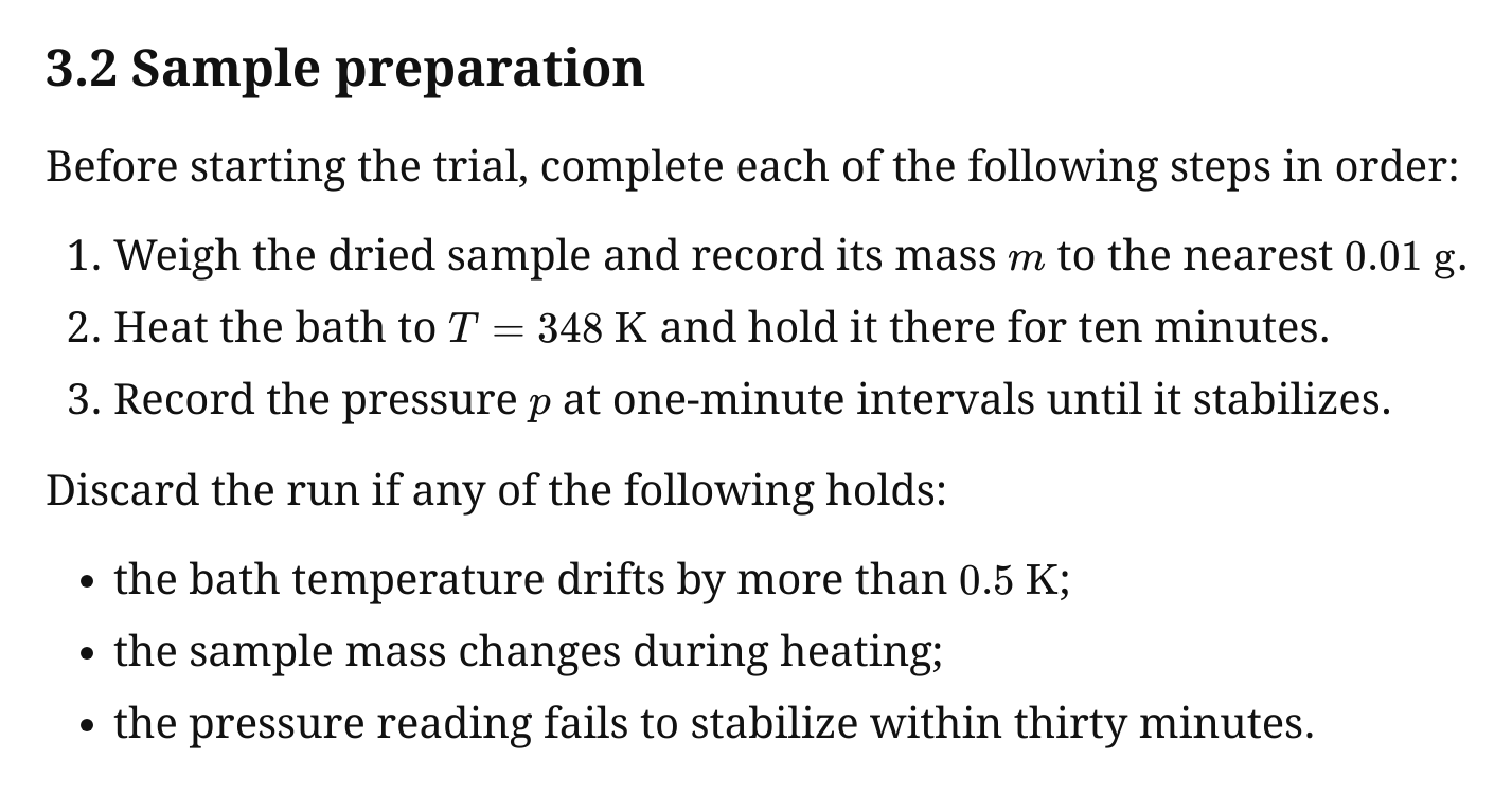
The option needs document layout, so both runs were sent with these options. The second run adds "disable_itemize": true.
{
  "src": "https://docs.mathpix.com/img/output-option-examples/list.png",
  "formats": [
    "text"
  ],
  "enable_document_layout": true
}
\subsection*{3.2 Sample preparation}

Before starting the trial, complete each of the following steps in order:
\begin{itemize}
\item[1.] Weigh the dried sample and record its mass \( m \) to the nearest 0.01 g .
\item[2.] Heat the bath to \( T=348 \mathrm{~K} \) and hold it there for ten minutes.
\item[3.] Record the pressure \( p \) at one-minute intervals until it stabilizes.
\end{itemize}

Discard the run if any of the following holds:
\begin{itemize}
\item[-] the bath temperature drifts by more than 0.5 K;
\item[-] the sample mass changes during heating;
\item[-] the pressure reading fails to stabilize within thirty minutes.
\end{itemize}
\subsection*{3.2 Sample preparation}

Before starting the trial, complete each of the following steps in order:
1. Weigh the dried sample and record its mass \( m \) to the nearest 0.01 g .
2. Heat the bath to \( T=348 \mathrm{~K} \) and hold it there for ten minutes.
3. Record the pressure \( p \) at one-minute intervals until it stabilizes.

Discard the run if any of the following holds:
- the bath temperature drifts by more than 0.5 K;
- the sample mass changes during heating;
- the pressure reading fails to stabilize within thirty minutes.
disable_lstlisting
Recognized pseudocode is returned inside an lstlisting environment by default, which lets the inline math in it render. With disable_lstlisting set, a standard fenced code block is returned instead, and math inside it stays plain LaTeX source.
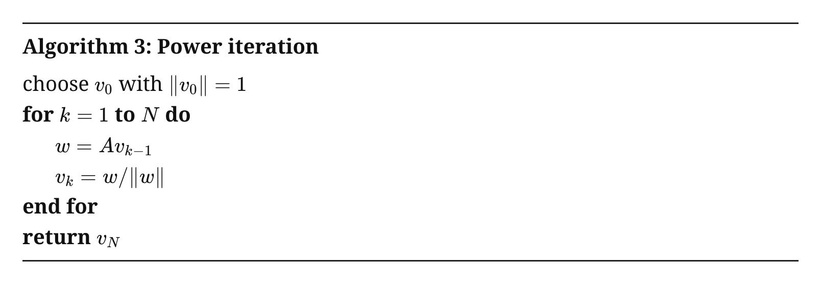
Both runs were sent with these options. The second run adds "disable_lstlisting": true.
{
  "src": "https://docs.mathpix.com/img/output-option-examples/algorithm.png",
  "formats": [
    "text"
  ],
  "enable_document_layout": true
}
\begin{lstlisting}[mathescape=true]
Algorithm 3: Power iteration
choose \( v_{0} \) with \( \left\|v_{0}\right\|=1 \)
for \( k=1 \) to \( N \) do
    \( w=A v_{k-1} \)
    \( v_{k}=w /\|w\| \)
end for
return \( v_{N} \)
\end{lstlisting}
```
Algorithm 3: Power iteration
choose \( v_{0} \) with \( \left\|v_{0}\right\|=1 \)
for \( k=1 \) to \( N \) do
    \( w=A v_{k-1} \)
    \( v_{k}=w /\|w\| \)
end for
return \( v_{N} \)
```
A listing that contains no math is returned as a fenced code block either way. The rendering requirement for lstlisting is stated with the parameter on the /v3/text reference.
include_page_info
The running head, the footer and the page number are included by default on /v3/text. With include_page_info set to false, they are dropped.
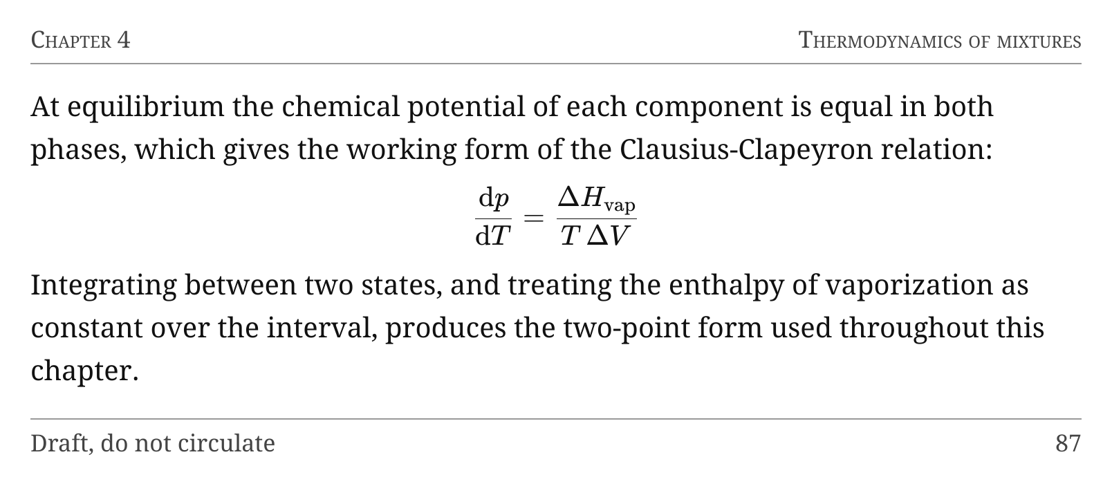
Both runs were sent with these options. The second run adds "include_page_info": false.
{
  "src": "https://docs.mathpix.com/img/output-option-examples/page.png",
  "formats": [
    "text"
  ],
  "enable_document_layout": true
}
Chapter 4
Thermodynamics of mixtures

At equilibrium the chemical potential of each component is equal in both phases, which gives the working form of the Clausius-Clapeyron relation:
\[
\frac{\mathrm{d} p}{\mathrm{~d} T}=\frac{\Delta H_{\text {vap }}}{T \Delta V}
\]
Integrating between two states, and treating the enthalpy of vaporization as constant over the interval, produces the two-point form used throughout this chapter.

Draft, do not circulate
87
At equilibrium the chemical potential of each component is equal in both phases, which gives the working form of the Clausius-Clapeyron relation:
\[
\frac{\mathrm{d} p}{\mathrm{~d} T}=\frac{\Delta H_{\text {vap }}}{T \Delta V}
\]
Integrating between two states, and treating the enthalpy of vaporization as constant over the interval, produces the two-point form used throughout this chapter.
The default differs by endpoint: page info is included by default on /v3/text and excluded by default on /v3/pdf, where documents usually carry running heads on every page. The option also accepts an array of page info types to keep only some of them; the accepted names are listed with the parameter on each endpoint page.
Math formatting options
The five options in this section reshape the LaTeX inside equations rather than the structure of the document, so they share one input image and one default output. Each subsection shows only the run with the option set.
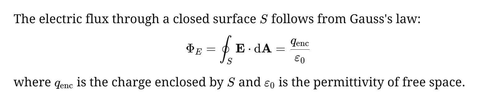
The default run was sent with these options. Each subsection states what its run adds.
{
  "src": "https://docs.mathpix.com/img/output-option-examples/formula.png",
  "formats": [
    "text"
  ]
}
The electric flux through a closed surface \( S \) follows from Gauss's law:
\[
\Phi_{E}=\oint_{S} \mathbf{E} \cdot \mathrm{~d} \mathbf{A}=\frac{q_{\mathrm{enc}}}{\varepsilon_{0}}
\]
where \( q_{\text {enc }} \) is the charge enclosed by \( S \) and \( \varepsilon_{0} \) is the permittivity of free space.
rm_spaces
rm_spaces is true by default and removes the white space between tokens inside equations. With "rm_spaces": false, that spacing is kept.
The electric flux through a closed surface \( S \) follows from Gauss's law:
\[
\Phi _ { E } = \oint _ { S } \mathbf { E } \cdot \mathrm {~d} \mathbf { A } = \frac { q _ { \mathrm { enc } } } { \varepsilon _ { 0 } }
\]
where \( q _ { \text {enc } } \) is the charge enclosed by \( S \) and \( \varepsilon _ { 0 } \) is the permittivity of free space.
rm_fonts
rm_fonts removes font commands such as \mathbf and \mathrm from equations. With "rm_fonts": true, the bold face that distinguished the vector from a scalar is gone from the output.
The electric flux through a closed surface \( S \) follows from Gauss's law:
\[
\Phi_{E}=\oint_{S} E \cdot d A =\frac{q_{enc}}{\varepsilon_{0}}
\]
where \( q_{\text {enc }} \) is the charge enclosed by \( S \) and \( \varepsilon_{0} \) is the permittivity of free space.
idiomatic_braces
idiomatic_braces drops the braces around single-character arguments, so x_{0} becomes x_0. With "idiomatic_braces": true, the LaTeX is equivalent and shorter. This option is accepted by /v3/text only.
The electric flux through a closed surface \( S \) follows from Gauss's law:
\[
\Phi_E=\oint_S \mathbf{E} \cdot \mathrm{~d} \mathbf{A}=\frac{q_{\mathrm{enc}}}{\varepsilon_0}
\]
where \( q_{\text {enc }} \) is the charge enclosed by \( S \) and \( \varepsilon_0 \) is the permittivity of free space.
math_inline_delimiters
math_inline_delimiters sets the pair of strings wrapped around inline math. The default is \( and \). This run adds "math_inline_delimiters": ["$", "$"].
The electric flux through a closed surface $S$ follows from Gauss's law:
\[
\Phi_{E}=\oint_{S} \mathbf{E} \cdot \mathrm{~d} \mathbf{A}=\frac{q_{\mathrm{enc}}}{\varepsilon_{0}}
\]
where $q_{\text {enc }}$ is the charge enclosed by $S$ and $\varepsilon_{0}$ is the permittivity of free space.
math_display_delimiters
math_display_delimiters sets the pair of strings wrapped around display math. The default is \[ and \], each on its own line. This run adds "math_display_delimiters": ["$$", "$$"], and the equation is returned on one line between the two markers.
The electric flux through a closed surface \( S \) follows from Gauss's law:
$$\Phi_{E}=\oint_{S} \mathbf{E} \cdot \mathrm{~d} \mathbf{A}=\frac{q_{\mathrm{enc}}}{\varepsilon_{0}}$$
where \( q_{\text {enc }} \) is the charge enclosed by \( S \) and \( \varepsilon_{0} \) is the permittivity of free space.
idiomatic_eqn_arrays
A group of related equations is returned in an array environment by default. With idiomatic_eqn_arrays set, the environment a person would write by hand is returned instead: cases for a piecewise definition, aligned or gathered for a list of equations.
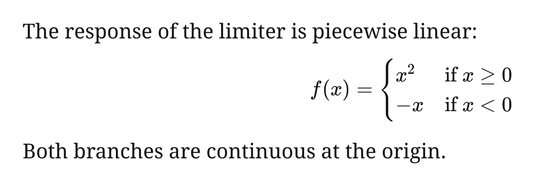
Both runs were sent with these options. The second run adds "idiomatic_eqn_arrays": true.
{
  "src": "https://docs.mathpix.com/img/output-option-examples/piecewise.png",
  "formats": [
    "text"
  ]
}
The response of the limiter is piecewise linear:
\[
f(x)=\left\{\begin{array}{ll}
x^{2} & \text { if } x \geq 0 \\
-x & \text { if } x<0
\end{array}\right.
\]

Both branches are continuous at the origin.
The response of the limiter is piecewise linear:
\[
f(x)= \begin{cases}x^{2} & \text { if } x \geq 0 \\ -x & \text { if } x<0\end{cases}
\]

Both branches are continuous at the origin.
include_equation_tags
An equation number printed beside a displayed equation is left out of the equation by default. With include_equation_tags set, it is returned as a \tag inside an equation* environment. Setting this option also turns on idiomatic_eqn_arrays.
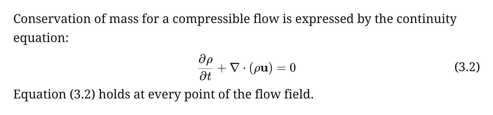
Both runs were sent with these options. The second run adds "include_equation_tags": true.
{
  "src": "https://docs.mathpix.com/img/output-option-examples/tagged.png",
  "formats": [
    "text"
  ]
}
Conservation of mass for a compressible flow is expressed by the continuity equation:
\[
\frac{\partial \rho}{\partial t}+\nabla \cdot(\rho \mathbf{u})=0
\]

Equation (3.2) holds at every point of the flow field.
Conservation of mass for a compressible flow is expressed by the continuity equation:
\[
\begin{equation*}
\frac{\partial \rho}{\partial t}+\nabla \cdot(\rho \mathbf{u})=0 \tag{3.2}
\end{equation*}
\]

Equation (3.2) holds at every point of the flow field.
numbers_default_to_math
A number sitting in running text is returned as text by default. With numbers_default_to_math set, the number is returned inside math delimiters; the unit that follows it stays text.
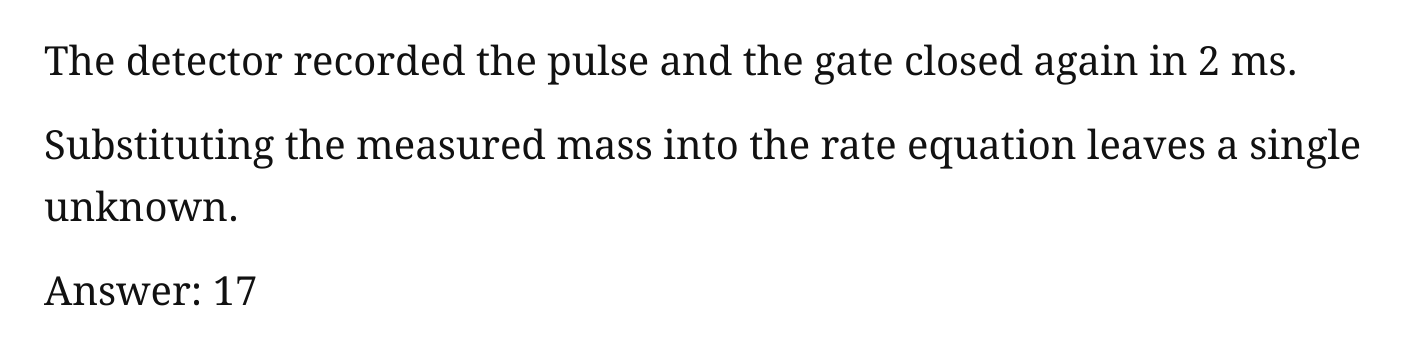
Both runs were sent with these options. The second run adds "numbers_default_to_math": true.
{
  "src": "https://docs.mathpix.com/img/output-option-examples/sentence.png",
  "formats": [
    "text"
  ]
}
The detector recorded the pulse and the gate closed again in 2 ms. Substituting the measured mass into the rate equation leaves a single unknown.

Answer: 17
The detector recorded the pulse and the gate closed again in \( 2 \) ms. Substituting the measured mass into the rate equation leaves a single unknown.

Answer: \( 17 \)
fullwidth_punctuation
For East Asian text, punctuation is returned as fullwidth characters by default, decided from the image content. With "fullwidth_punctuation": false, the same marks are returned as halfwidth ASCII punctuation.
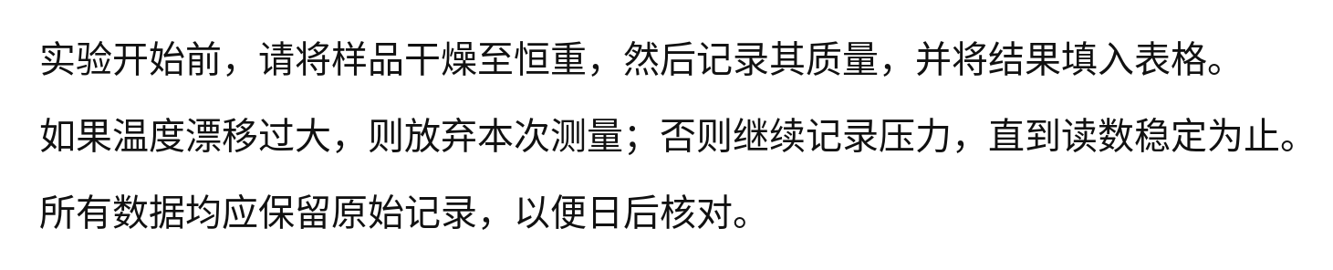
Both runs were sent with these options. The second run adds "fullwidth_punctuation": false.
{
  "src": "https://docs.mathpix.com/img/output-option-examples/cjk.png",
  "formats": [
    "text"
  ]
}
实验开始前,请将样品干燥至恒重,然后记录其质量,并将结果填入表格。如果温度漂移过大,则放弃本次测量;否则继续记录压力,直到读数稳定为止。所有数据均应保留原始记录,以便日后核对。
实验开始前, 请将样品干燥至恒重, 然后记录其质量, 并将结果填入表格。如果温度漂移过大, 则放弃本次测量; 否则继续记录压力, 直到读数稳定为止。所有数据均应保留原始记录, 以便日后核对。
include_smiles
On /v3/text, a chemical diagram is left out of the output by default. With include_smiles set, it is returned as a <smiles> element holding the structure as a SMILES string. On /v3/pdf the option is on by default, as the document examples below show.
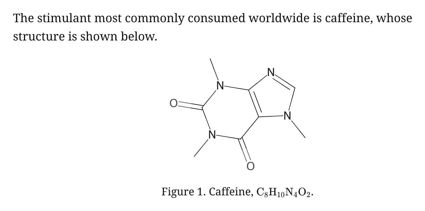
Both runs were sent with these options. The second run adds "include_smiles": true.
{
  "src": "https://docs.mathpix.com/img/output-option-examples/molecule.png",
  "formats": [
    "text"
  ]
}
The stimulant most commonly consumed worldwide is caffeine, whose structure is shown below.

Figure 1. Caffeine, \( \mathrm{C}_{8} \mathrm{H}_{10} \mathrm{~N}_{4} \mathrm{O}_{2} \).
The stimulant most commonly consumed worldwide is caffeine, whose structure is shown below.
<smiles>Cn1c(=O)c2c(ncn2C)n(C)c1=O</smiles>

Figure 1. Caffeine, \( \mathrm{C}_{8} \mathrm{H}_{10} \mathrm{~N}_{4} \mathrm{O}_{2} \).
include_inchi
include_inchi adds inchi and inchi_key attributes to each <smiles> element. It only applies when include_smiles is on, so both runs of this pair were sent with "include_smiles": true, and the second adds "include_inchi": true. The input image is the one pictured under include_smiles. This option is accepted by /v3/text only.
{
  "src": "https://docs.mathpix.com/img/output-option-examples/molecule.png",
  "formats": [
    "text"
  ],
  "include_smiles": true
}
The stimulant most commonly consumed worldwide is caffeine, whose structure is shown below.
<smiles>Cn1c(=O)c2c(ncn2C)n(C)c1=O</smiles>

Figure 1. Caffeine, \( \mathrm{C}_{8} \mathrm{H}_{10} \mathrm{~N}_{4} \mathrm{O}_{2} \).
The stimulant most commonly consumed worldwide is caffeine, whose structure is shown below.
<smiles inchi="InChI=1S/C8H10N4O2/c1-10-4-9-6-5(10)7(13)12(3)8(14)11(6)2/h4H,1-3H3" inchi_key="RYYVLZVUVIJVGH-UHFFFAOYSA-N">Cn1c(=O)c2c(ncn2C)n(C)c1=O</smiles>

Figure 1. Caffeine, \( \mathrm{C}_{8} \mathrm{H}_{10} \mathrm{~N}_{4} \mathrm{O}_{2} \).
Document options on POST /v3/pdf
The options in this section exist on /v3/pdf only, because they concern pages, links and section structure rather than a single image. The table above identifies which image options are also accepted by /v3/pdf, where they apply to the whole document; document layout is always on there, so enable_document_layout is not needed.
The examples use a two page PDF, document.pdf, with numbered sections, two links and a chemical diagram.
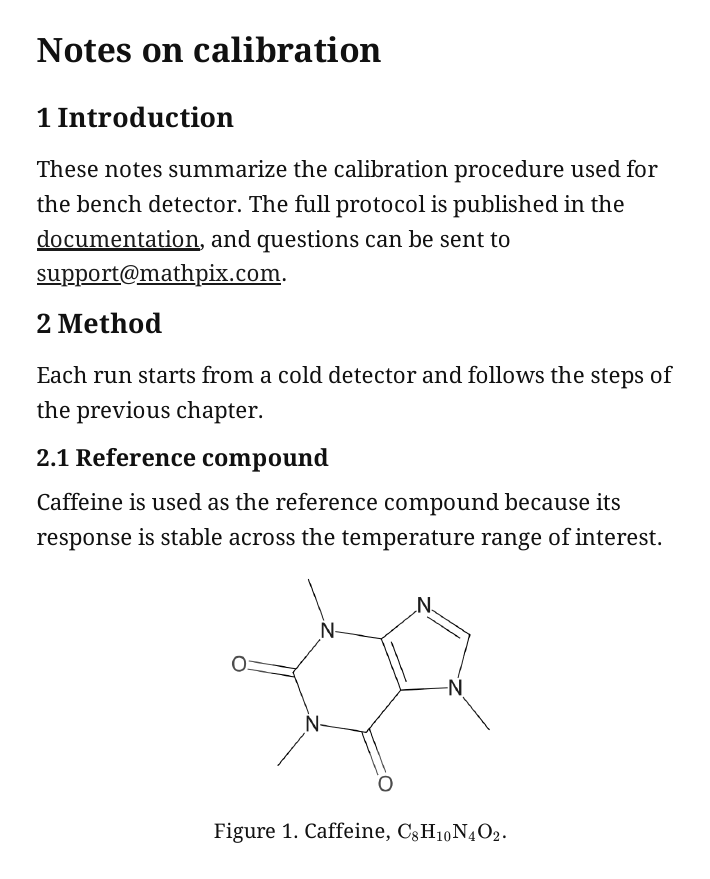
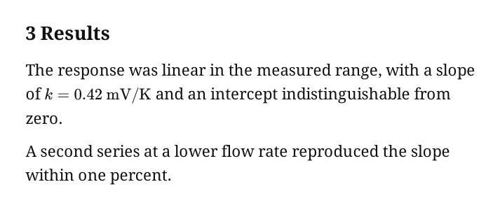
The document was submitted with no options, and the .mmd result was fetched once processing completed. Each subsection states the option its run adds.
{
  "url": "https://docs.mathpix.com/files/output-option-examples/document.pdf"
}
\section*{Notes on calibration}

\section*{1 Introduction}

These notes summarize the calibration procedure used for the bench detector. The full protocol is published in the documentation, and questions can be sent to support@mathpix.com.

\section*{2 Method}

Each run starts from a cold detector and follows the steps of the previous chapter.

\subsection*{2.1 Reference compound}

Caffeine is used as the reference compound because its response is stable across the temperature range of interest.
<smiles>Cn1c(=O)c2c(ncn2C)n(C)c1=O</smiles>

Figure 1. Caffeine, \(\mathrm{C}_{8} \mathrm{H}_{10} \mathrm{~N}_{4} \mathrm{O}_{2}\).

\section*{3 Results}

The response was linear in the measured range, with a slope of \(k=0.42 \mathrm{mV} / \mathrm{K}\) and an intercept indistinguishable from zero.

A second series at a lower flow rate reproduced the slope within one percent.
include_page_breaks
With "include_page_breaks": true, each page's output ends with a \pagebreak line, so a two page document carries two markers.
\section*{Notes on calibration}

\section*{1 Introduction}

These notes summarize the calibration procedure used for the bench detector. The full protocol is published in the documentation, and questions can be sent to support@mathpix.com.

\section*{2 Method}

Each run starts from a cold detector and follows the steps of the previous chapter.

\subsection*{2.1 Reference compound}

Caffeine is used as the reference compound because its response is stable across the temperature range of interest.
<smiles>Cn1c(=O)c2c(ncn2C)n(C)c1=O</smiles>

Figure 1. Caffeine, \(\mathrm{C}_{8} \mathrm{H}_{10} \mathrm{~N}_{4} \mathrm{O}_{2}\).
\pagebreak


\section*{3 Results}

The response was linear in the measured range, with a slope of \(k=0.42 \mathrm{mV} / \mathrm{K}\) and an intercept indistinguishable from zero.

A second series at a lower flow rate reproduced the slope within one percent.
\pagebreak
include_hyperlinks
With "include_hyperlinks": true, the anchor text of each link stored in the PDF becomes a Markdown link to the stored target. Only http, https and mailto links are preserved.
\section*{Notes on calibration}

\section*{1 Introduction}

These notes summarize the calibration procedure used for the bench detector. The full protocol is published in the [documentation](https://mathpix.com/docs), and questions can be sent to [support@mathpix.com](mailto:support@mathpix.com).

\section*{2 Method}

Each run starts from a cold detector and follows the steps of the previous chapter.

\subsection*{2.1 Reference compound}

Caffeine is used as the reference compound because its response is stable across the temperature range of interest.
<smiles>Cn1c(=O)c2c(ncn2C)n(C)c1=O</smiles>

Figure 1. Caffeine, \(\mathrm{C}_{8} \mathrm{H}_{10} \mathrm{~N}_{4} \mathrm{O}_{2}\).

\section*{3 Results}

The response was linear in the measured range, with a slope of \(k=0.42 \mathrm{mV} / \mathrm{K}\) and an intercept indistinguishable from zero.

A second series at a lower flow rate reproduced the slope within one percent.
include_chemistry_as_image
With "include_chemistry_as_image": true, a chemical diagram is returned as an image crop hosted by Mathpix, with the SMILES string in the alt text, instead of an inline <smiles> element.
\section*{Notes on calibration}

\section*{1 Introduction}

These notes summarize the calibration procedure used for the bench detector. The full protocol is published in the documentation, and questions can be sent to support@mathpix.com.

\section*{2 Method}

Each run starts from a cold detector and follows the steps of the previous chapter.

\subsection*{2.1 Reference compound}

Caffeine is used as the reference compound because its response is stable across the temperature range of interest.

\begin{figure}
\includegraphics[alt={<smiles>Cn1c(=O)c2c(ncn2C)n(C)c1=O</smiles>},max width=\textwidth]{https://cdn.mathpix.com/cropped/2024_01_01_abcdef0123456789abcdg-1.jpg?height=493&width=597&top_left_y=1565&top_left_x=765}
\captionsetup{labelformat=empty}
\caption{Figure 1. Caffeine, \(\mathrm{C}_{8} \mathrm{H}_{10} \mathrm{~N}_{4} \mathrm{O}_{2}\).}
\end{figure}

\section*{3 Results}

The response was linear in the measured range, with a slope of \(k=0.42 \mathrm{mV} / \mathrm{K}\) and an intercept indistinguishable from zero.

A second series at a lower flow rate reproduced the slope within one percent.
remove_section_numbering
Numbers printed in section headings are kept by default, which is what preserve_section_numbering being true means. With "remove_section_numbering": true, the printed numbers are dropped from the headings.
\section*{Notes on calibration}

\section*{Introduction}

These notes summarize the calibration procedure used for the bench detector. The full protocol is published in the documentation, and questions can be sent to support@mathpix.com.

\section*{Method}

Each run starts from a cold detector and follows the steps of the previous chapter.

\subsection*{Reference compound}

Caffeine is used as the reference compound because its response is stable across the temperature range of interest.
<smiles>Cn1c(=O)c2c(ncn2C)n(C)c1=O</smiles>

Figure 1. Caffeine, \(\mathrm{C}_{8} \mathrm{H}_{10} \mathrm{~N}_{4} \mathrm{O}_{2}\).

\section*{Results}

The response was linear in the measured range, with a slope of \(k=0.42 \mathrm{mV} / \mathrm{K}\) and an intercept indistinguishable from zero.

A second series at a lower flow rate reproduced the slope within one percent.
auto_number_sections
auto_number_sections numbers the sections of a document that has none. The example uses a second PDF, unnumbered.pdf, whose headings carry no numbers.
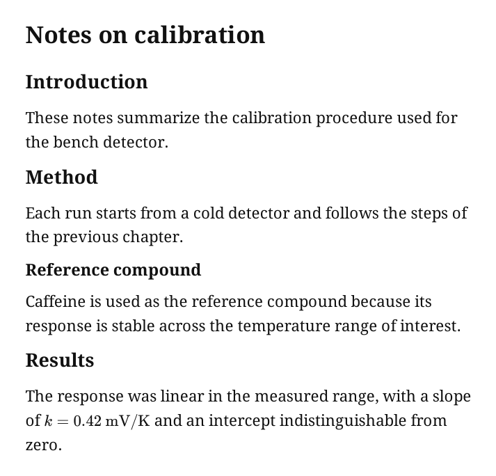
{
  "url": "https://docs.mathpix.com/files/output-option-examples/unnumbered.pdf"
}
\section*{Notes on calibration}

\section*{Introduction}

These notes summarize the calibration procedure used for the bench detector.

\section*{Method}

Each run starts from a cold detector and follows the steps of the previous chapter.

\section*{Reference compound}

Caffeine is used as the reference compound because its response is stable across the temperature range of interest.

\section*{Results}

The response was linear in the measured range, with a slope of \(k=0.42 \mathrm{mV} / \mathrm{K}\) and an intercept indistinguishable from zero.
With "auto_number_sections": true, the headings are returned as numbered \section commands instead of unnumbered \section* commands, and the numbers are assigned by the renderer.
\section{Notes on calibration}

\section{Introduction}

These notes summarize the calibration procedure used for the bench detector.

\section{Method}

Each run starts from a cold detector and follows the steps of the previous chapter.

\section{Reference compound}

Caffeine is used as the reference compound because its response is stable across the temperature range of interest.

\section{Results}

The response was linear in the measured range, with a slope of \(k=0.42 \mathrm{mV} / \mathrm{K}\) and an intercept indistinguishable from zero.
Only one of auto_number_sections, remove_section_numbering and preserve_section_numbering can be true in a request. Setting one of the first two does not require turning off the default, as these runs show.